Overview
An end-to-end macroeconomic forecasting system built to compete in the Macro Forecasting Challenge, a national university tournament organized by Banco de Occidente and Occieconómicas. The pipeline forecasts 10 financial and macroeconomic variables for Colombia and international markets, scored against realized data using a weighted relative-error metric.
Repository: github.com/RedFoxRising/macro-forecasting-occidente
Competition: Banco de Occidente × Occieconómicas — 2026
The Problem
The challenge required forecasting 10 variables simultaneously, each from a different official source, at different frequencies, and with different statistical behaviors. A single modeling approach wouldn’t work — a method suited to an equity index is wrong for inflation, and vice versa. The real problem was building a unified pipeline that handles all of them cleanly while staying fast enough to update and resubmit each month.
Tech Stack
- Language: Python (Google Colab)
- Data:
yfinance,requests(Datos Abiertos API), DANE Excel files, BanRep SUAMECA, Investing.com CSV - Modeling:
statsmodels(SARIMAX, AutoReg),scikit-learn(LinearRegression) - Processing:
pandas,numpy - Visualization:
matplotlib
Variables and Models
| Variable | Weight | Model |
|---|---|---|
| Colombian inflation (monthly %) | 15% | SARIMA(1,1,1)(1,1,1,12) |
| USD/COP exchange rate (TRM) | 10% | Random walk + drift |
| ISE economic tracking index | 10% | AR(2) |
| 10-year TES bond yield | 10% | Linear regression vs UST10Y |
| Colcap equity index | 10% | Random walk + drift |
| S&P 500 | 10% | Random walk + drift |
| Monetary policy rate (BanRep) | 10% | Rule-based heuristic |
| National unemployment rate | 10% | SARIMA(1,1,0)(0,1,1,12) |
| Brent crude | 5% | Random walk + drift |
| Gold | 5% | Random walk + drift |
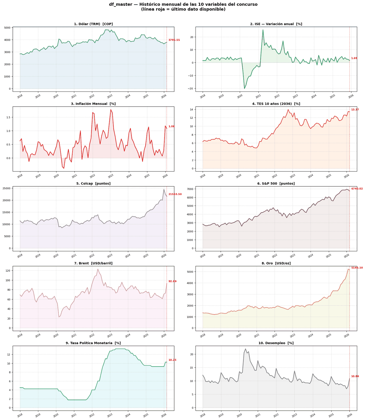
The unified df_master: ten sources, six formats, one monthly index. Tap to enlarge.
Pipeline
Extraction. Six sources, each with its own parser. Market prices come from Yahoo Finance via yfinance. The TRM comes from the official Datos Abiertos API — the same series the competition uses to score submissions. Inflation, the ISE, and unemployment come from DANE spreadsheets; the policy rate from BanRep’s SUAMECA system; the TES yield from an Investing.com export.
Unification. All series are aligned into a single monthly DataFrame covering 2018 onward. Market variables are resampled with resample('BME').last() to take the last business day of each month; flow variables are indexed to first-of-month. Getting this convention wrong produces silently misaligned data that corrupts every model downstream.
Modeling. One model per variable, chosen by statistical behavior rather than sophistication. Five market prices use a drift-adjusted random walk; the two seasonal series use SARIMA; the ISE uses an AR(2); the TES yield is regressed against the US 10-year.
Manual review. Before submitting, every model output is checked against qualitative context and sanity-checked for units. Both halves of that layer earned their place in round one — see Results.
Validation
Every model was validated with walk-forward backtesting over 24 months (April 2024 – March 2026). For each test month, the model retrains using only data available before that month — no future observations leak into the training window, which a standard train/test split would allow.
| Variable | Weight | Model error | Random walk | Observations |
|---|---|---|---|---|
| TRM | 10% | 2.33% | 2.33% | 24 |
| ISE | 10% | 338.96% | 376.41% | 21 |
| Inflation | 15% | 52.84% | 85.02% | 23 |
| TES 10Y | 10% | 3.79% | 3.79% | 24 |
| Colcap | 10% | 3.64% | 3.64% | 24 |
| S&P 500 | 10% | 2.45% | 2.45% | 24 |
| Brent | 5% | 5.97% | 5.97% | 24 |
| Gold | 5% | 3.25% | 3.25% | 24 |
| Policy rate | 10% | 2.18% | 2.18% | 24 |
| Unemployment | 10% | 6.20% | 7.84% | 22 |
Two things this table says plainly.
First, the modeling only beat the naive benchmark on three variables — inflation, unemployment, and the ISE. The other seven show identical errors because those seven are random walks. That isn’t a shortcut; it’s the result of testing whether anything more elaborate helped, and finding it didn’t. At a one-month horizon on liquid markets, beating a random walk is genuinely hard.
Second, the ISE and inflation figures are metric artifacts, not model failures — see Challenge 1 below.
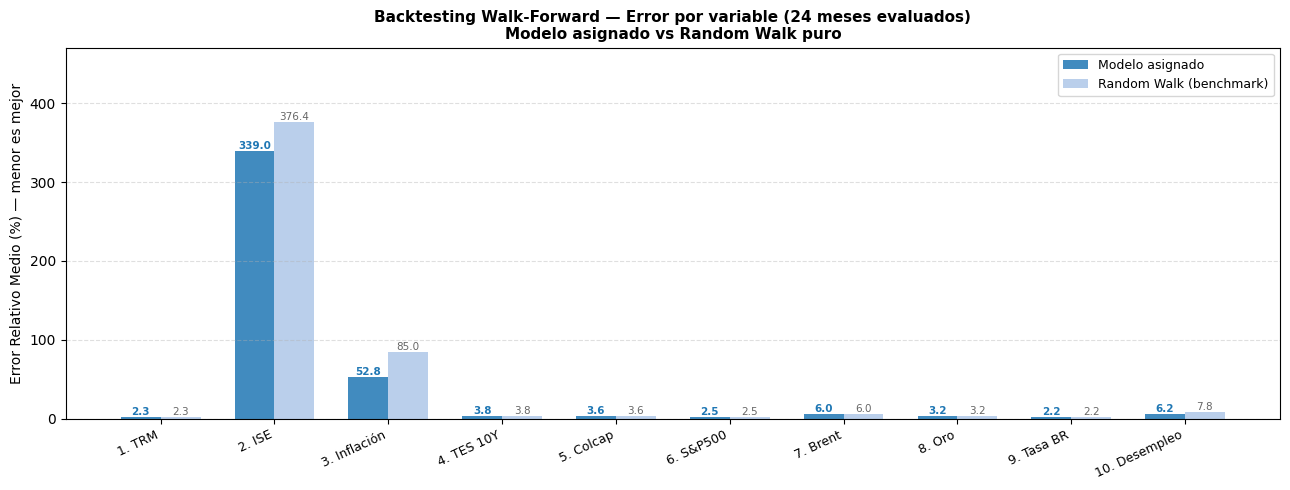
Assigned model vs. random walk benchmark. The bars are identical wherever the assigned model is a random walk. Tap to enlarge.
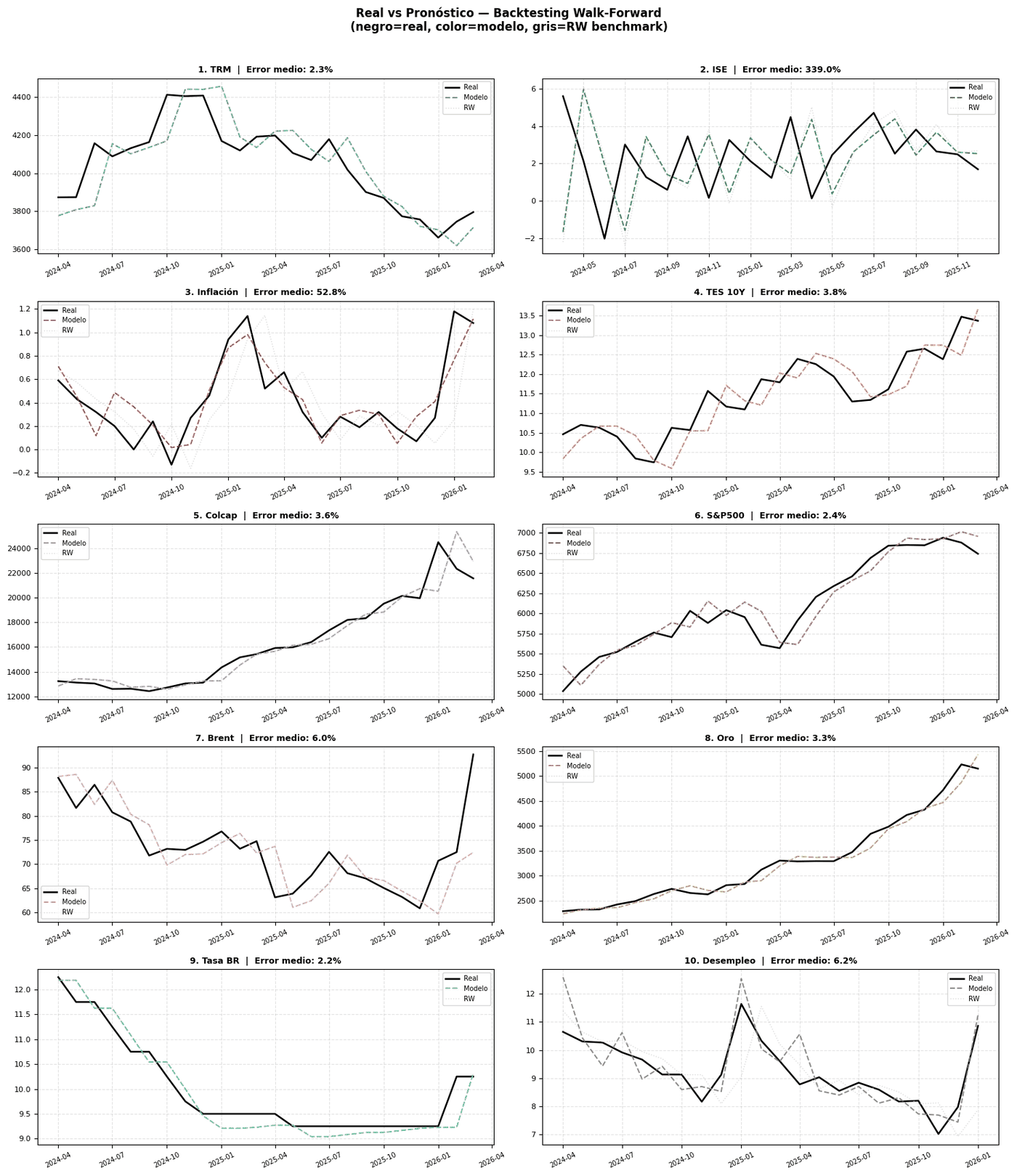
Realized vs. forecast, month by month, across the full walk-forward window. Tap to enlarge.
Challenges
Challenge 1 — Unstable error metric near zero.
The competition scores with |P−O|/O × 100, which explodes when the observed value approaches zero. Monthly inflation runs around 0.5%, and the ISE year-on-year change was near 0.13% in one month; a 0.5 pp absolute miss becomes a 380% relative error. Rather than assume the models had failed, I verified the units in the master DataFrame and confirmed the metric itself was the problem. The fix uses max(|O|, ε) as the denominator, with ε set to the 25th percentile of each variable’s historical absolute values — stabilizing the metric while leaving normal observations untouched.
Challenge 2 — Outliers in the TES series. The Investing.com export contained a digitization error producing a yield above 20%, historically impossible for Colombia. It’s detected against a plausibility threshold and replaced with linear interpolation between adjacent observations.
Challenge 3 — ISE extraction from a nested spreadsheet.
DANE’s ISE file packs several indicator tables into one sheet, with year columns carrying provisional labels like 2024p. The extractor locates the total-ISE row by indicator name and detects year columns by testing whether the first four characters are digits, which survives DANE’s periodic format changes.
Results — Round 1
The manual layer worked twice
On the TRM, judgment beat the model. Reserve levels and the debt trajectory pointed to a weaker peso than the consensus expected, so the submission went in at 3,690 instead of the model’s 3,762.
| TRM forecast | Value | Error vs 3,670 |
|---|---|---|
| Model output (random walk + drift) | 3,762 | 2.51% |
| Competition consensus | 3,757 | 2.37% |
| Submitted (manual adjustment) | 3,690 | 0.55% |
It was the most accurate TRM forecast of the round.
On the Colcap, review caught a unit error. The pipeline pulled ICOLCAP.CL from Yahoo Finance — the ETF, not the index — producing a forecast an order of magnitude off the scale the competition scores against. Nothing failed; the number simply flowed through the pipeline looking plausible. It was caught in manual review and the equivalent index value was submitted instead. A wrong ticker that raises no exception is the kind of bug that survives every automated check.
Three ways the models missed
The variables that went wrong went wrong for three different reasons, and the distinction matters more than the errors themselves.
Discrete decisions. The heuristic projected the policy rate unchanged at 10.25%; BanRep raised to 11.25%. Realized error 8.89%, against a consensus error of 6.67% — and roughly four times what 24 months of walk-forward validation suggested for that variable. No time series contains a rate decision that hasn’t happened yet.
Exogenous shocks. Brent was forecast at 94.20 and closed at 118. The war in Iran is not in the historical series, and no amount of backtesting would have surfaced it.
Drift in a volatile regime. Gold sat near 5,000 at submission time. We expected the rally to continue but decelerate, and forecast 5,314.70; the month reversed and it closed at 4,648. The drift term extrapolates recent trend — which in a rally means betting the trend holds. The pure random walk, anchored at the starting level, would have landed closer. This is not a bug; it is the model’s assumption doing exactly what it promises.
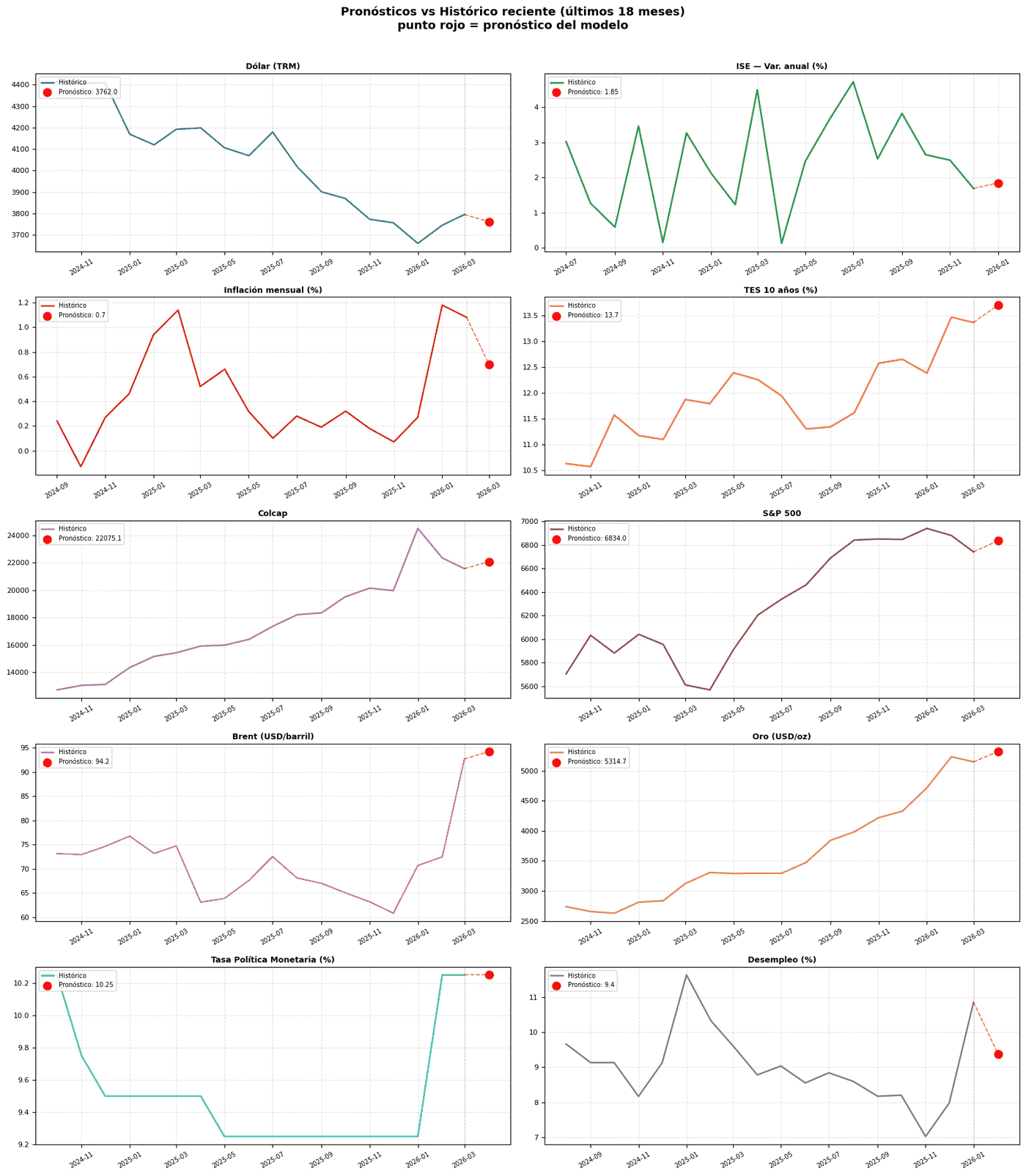
Round 1 submissions against recent history. Tap to enlarge.
What I Learned
Not every variable is the same forecasting problem
Going in, I treated the ten variables as one task with ten instances: pull the data, match a model to the statistical behavior, validate, submit. The results showed they fall into three groups that barely belong together.
Some are continuous and reasonably stable. The TRM, the TES yield, the S&P 500 — for these the pipeline did what a pipeline should. Others are driven by a discrete decision or an external event. The policy rate is set by seven people in a room; Brent responded to a war. No amount of history contains a decision that hasn’t been made yet, and fitting a smooth model to a variable that moves in steps produces a number that looks like a forecast without being one. A third group is continuous but was passing through a volatile regime. Gold was mid-rally, and the drift term reads recent trend as information about the future — which is a bet that the trend holds. When the month reversed, the drift is what carried us further from the answer than a naive random walk would have.
The practical consequence is that these should not share a method. Statistical forecasting is the right tool for the first group. The second needs weighted scenarios and an explicit view on what each actor is likely to do. Treating them identically is how you end up reporting a policy-rate forecast with the same implied confidence as an equity index.
What a backtest cannot tell you
My walk-forward validation put the policy rate at a 2.18% mean error — second lowest of the ten variables. The realized error was 8.89%. That gap is the most useful thing I took away from this project.
The validation window ran from April 2024 to March 2026. In those 24 months, BanRep moved gradually and predictably, so the heuristic tracked it well. The backtest was not wrong; it was answering a narrower question than I thought it was. A low mean error can mean the model is good, or it can mean the window contained nothing hard — and the output looks identical either way.
That distinction matters beyond this competition. Validation tells you how a model performed against the past it was shown, not how it will perform against a future that differs structurally from that past. I now think the useful question is not “what was the mean error” but “what was the hardest thing in the window, and did the model handle it.” If the answer is that nothing hard happened, the error figure is describing the sample, not the model.
The best call and the worst one came from the same place
On the TRM we did not take the model’s output. Reserve levels and the debt trajectory suggested the peso was under more pressure than the consensus was pricing, so we adjusted the submission downward. It was the most accurate TRM forecast of the round, and roughly four times better than what the model alone would have produced.
On the policy rate we let the heuristic run untouched.
What bothers me is that the same reasoning applied. A scenario of currency and fiscal stress is precisely a scenario in which a central bank tightens. We had the analysis, and we had already decided it was strong enough to override a model. We simply did not carry it across to the variable where it mattered most — arguably because forecasting an exchange rate felt like something I could have a view on, and forecasting a central bank’s decision did not.
The lesson is not that models fail. It is that discretionary judgment has to be applied to the whole set or to none of it. Applying it only where you feel qualified to hold an opinion means your errors concentrate exactly where you were least willing to think.
Round one also happened to contain three exogenous shocks in a single month — the conflict in Iran, the escalation between the executive and the central bank, and a reversal in metals. That explains the size of the misses. It does not explain away the one that mattered, which was a failure of process rather than of luck.
Parsing real-world official data
Government sources are not clean. DANE’s inflation file uses a wide layout (years as columns, months as rows) that has to be melted before it’s usable. The BanRep export carries logos and footnotes above the data. Each source needed its own extraction function with format-specific logic — and every hour spent making one robust paid off in every subsequent month.
Honest backtesting, and its limits
Walk-forward validation is the right way to test a time-series model, and it did its job: it showed which models were genuinely predictive and which only looked good in-sample. But a backtest can only test against what happened in its window. That distinction turned out to matter more than the methodology itself.
When simple beats complex
For the five market-price variables, a drift-adjusted random walk matched everything more sophisticated I tried. That’s the expected result for efficient markets at a one-month horizon, and a reminder that complexity is not quality.
Future Improvements
- Add the SIPSA food price index as an external regressor for inflation (SARIMAX)
- Add XM energy consumption data as a proxy for the ISE
- Build a scenario module (bear / base / bull) with probability weighting
- Split the variable set explicitly: statistical forecasting for continuous series, weighted scenarios for anything driven by a discrete decision
- Add automated unit and scale assertions so ticker mismatches fail loudly
- Automate the data refresh so the pipeline runs without manual downloads